一类四阶非线性时间分数阶双曲方程的L2-1σ 有限元方法
王岩, 杨益宁*
(内蒙古大学数学科学学院, 呼和浩特 010021)
摘要: 本文针对一类四阶非线性时间分数阶双曲方程构造了一种具有时空二阶精度的数值算法。首先引入一个低阶参数β=α-1将一个α ∈ (1, 2) 的Caputo分数阶导数降为β∈ (0, 1) 的Caputo分数阶导数, 其次引入两个辅助函数变量v=ut , ζ=Δu将四阶非线性时间分数阶双曲方程转化为一个包含积分项的低阶非线性耦合系统。在时间方向上利用L2-1σ公式对其分数阶导数项进行离散, 同时利用复化梯形公式离散积分项, 在空间上采用传统Galerkin有限元方法, 进一步得到该低价非线性耦合系统的全离散有限元格式。以二维区域上的均匀矩形剖分为例, 利用双线性基函数给出了刚度矩阵和荷载矩阵的具体形式, 得到了全离散数值格式的详细算法实现过程。最后分别对一维和二维算例进行数值模拟, 对比于原方程该低阶系统能够同时观察三个未知量u, v, ζ的变化, 并且详细地列出不同参数和不同时空步长下这三个未知量的误差、图像和收敛阶, 充分地验证了该算法的可行性和有效性。
关键词: 四阶非线性时间分数阶双曲方程, L2-1σ , 有限元方法
DOI: 10.48014/fcpm.20240410001
引用格式: 王岩, 杨益宁. 一类四阶非线性时间分数阶双曲方程的L2-1σ 有限元方法[J]. 中国理论数学前沿, 2024, 2(2): 16-26.
文章类型: 研究性论文
收稿日期: 2024-04-10
接收日期: 2024-04-19
出版日期: 2024-06-28
1 引言
近年来,由于具有空间四阶导数的时间分数阶偏微分方程能够描述许多实际问题而得到各领域学者的广泛关注,其中包括四阶时间分数阶波动方程[1-3],四阶时间分数阶扩散方程[4-6],四阶分数阶积分-微分方程[7]等。由于方程自身的结构复杂性,传统的解析方法很难找到其精确解,故对于有效的数值方法的研究变得至关重要。这里我们主要关注离散四阶时间分数阶偏微分方程的各类数值方法。Wang等[8]采用修正L1 Crank-Nicolson有限元法求解了二维非线性四阶时间分数阶扩散波方程,同时进行了稳定性分析和最优L2范数误差估计,并通过数值模拟验证了该方法的可行性。文献[9]介绍了多维情况下时间分数阶四阶反应扩散模型的混合无网格方法,并且给出了一维、二维和三维不同几何域的算例。文献[11]构造了一个有效的二维非线性四阶分数阶波动方程的二阶时间精度数值算法,并在矩形和圆形空间域上进行了数值实验验证了算法的有效性和收敛效率。文献[12]提出了求解二维非线性四阶时间分数阶波模型的WSGD 有限元法,进一步利用时空分裂技术,在不限制空间网格大小与时间步长关系的情况下推导了无条件最优误差估计和稳定性结果,最后通过光滑解和非光滑解进行数值计算验证了理论结果的正确性。在文献[13]中,主要研究了二维分布阶时间分数阶四阶偏微分方程的时空Petrov-Galerkin谱方法,给出了光滑解和有限正则解的例子,数值证明了所提方法的高效性、精确性和指数收敛性。
在本文中,我们主要考虑L2-1σ有限元方法数值求解下列四阶非线性时间分数阶双曲方程
 u+Δ2u-Δu+f(u)=g(x,t),(1)
其中(x,t)∈Ω×J,时间区域为J=(0,1],Ω⊂ 具有光滑边界 ∂Ω 的凸多边形区域。该方程初边值条件分别为
u(x,t)=Δu(x,t)=0,(x,t)∈∂Ω× ,
,
u(x,0)=0, (x,0)=u1(x),x∈
 .
.
初值u1(x)和源项g(x,t)均为光滑函数。非线性f(u)属于C2(R)且为多项式函数或有界函数。α∈(1,2)时Caputo分数阶导数定义为
 (2)
(2)
在本文中,针对四阶非线性时间分数阶双曲方程,通过引入新的阶数β=α-1和两个中间变量 v=ut,ζ=Δu,将原四阶问题改写为一个低阶的耦合系统。结合L2-1σ格式近似时间方向,结合传统Galerkin有限元方法离散空间方向,进一步得到低阶耦合系统的全离散有限元格式。以二维正方形空间区域为例,通过双线性基函数给出数值格式的详细算法过程,即刚度矩阵和荷载矩阵的具体形式。最后,利用MATLAB分别模拟了一维和二维算例,并记录了不同时空步长条件下的误差数据以及收敛阶,也通过等高线图刻画了不同参数下误差的形态。
本文剩余部分结构如下:在第二节中我们构造了一个L2-1σ有限元全离散数值格式。在第三节中给出了算法的详细过程。在第四节中通过两个数值算例验证了该算法的有效性。在第五节中对本文进行简短的总结。
2 数值格式
首先引入参数β=α-1和中间变量v=ut,ζ=Δu,将方程(1)改写为如下低阶耦合系统
 (3)
(3)
为了建立全离散格式,我们首先对时间区域[0,T]进行均匀划分,插入节点tn=nΔt(n=0,1,2,…,N)且N为正整数,时间步长为Δt= .
.
其次引入时间离散格式的相关引理,其中σ=1- ,v(·,tn)=vn.
引理1[10] 在时间节点tn+σ处,关于时间一阶导数项 (tn+σ)有如下离散公式成立
(tn+σ)
=
∂tvn+σ+
引理2[10] 在时间节点tn+σ处,关于v(tn+σ)和非线性项f(v(tn+σ))有如下离散公式成立
v(tn+σ)=σvn+1+(1-σ)vn+O(Δt2),
vn+σ+O(Δt2), n≥0,
f(v(tn+σ))=
f(vn+σ)+
引理3[10] 在时间节点tn+σ处,关于时间分数阶导数项 v(tn+σ)的L2-1σ离散公式如下
v(tn+σ)
 vn+σ+O(Δt3-β).
其中当n≥1时,有
 =
=
当n=0时,有 =a0,
=a0,
a0=σ1-β,
ak=(k+σ)1-β-(k-1+σ)1-β, k≥1,
bk= ((k+σ)2-β-(k-1+σ)2-β)-
 ((k+σ)1-β+(k-1+σ)1-β), k≥1.
引理4[14] 在时间节点tn+σ处,关于时间积分项 的复化梯形离散公式如下
在上述离散公式的基础上可以得到方程(1)的时间离散格式
其中
 =[∂tun+σ-(tn+σ)]-
[vn+σ-v(tn+σ)]+O(Δt2),
 =[∂tζn+σ-
 (tn+σ)]-
[Δvn+σ-Δv(tn+σ)]+O(Δt2),
 =[∂tvn+σ-(tn+σ)]+[vn+σ-
v(tn+σ)]-[Λvn+σ- vdr]-
vdr]-
[Δvn+σ-Δv(tn+σ)]+[Δζn+σ-Δζ(tn+σ)]+
[f(vn+σ)-f(v(tn+σ))]+O(Δt2).
定义有限元空间
Wh={wh∈ (Ω), wh|e∈
 (x), e∈Th}.
设Th为区域Ω的一个拟一致剖分,(x)表示单元上关于x的次数不超过r的多项式集合。
进一步,可得有限元全离散格式,求 ,
, ,
, ∈Wh,使得
 (4)
(4)
3 算法实现
在这一部分中主要给出全离散格式(4)的详细计算过程。取定空间正方形区域Ω=[0,1]×[0,1],Th为该区域上的一个均匀矩形剖分,满足0=x0<x1<…<xM=1,0=y0<y1<…<yM=1,h=xi-xi-1=yi-yi-1= ,i=1,…,M.定义ei∈Th为一个矩形单元,Ni(x,y)为单元 ei上的形状函数向量。通过仿射变换,将矩形单元 ei变换为标准单元
 =[-1,1]×[-1,1],故标准单元上的形状函数向量为
N(ξ,η)= [(ξ-1)(η-1),-(ξ+1)(η-1),
(ξ+1)(η+1),-(ξ-1)(η+1)]T.
下面给出ei上的刚度矩阵和荷载矩阵

此外,其他小单元ei上的矩阵向量表示为
则K,A和G为对应的刚度矩阵和荷载矩阵,u0,F分别为初值和非线性项对应的矩阵形式。
那么全离散格式(4)可以写为如下的矩阵形式
PEn+1=H.
矩阵P,En+1,H分别为
P= ,
,
En+1= ,
,
H= .
.
其中
λ= ,
,
GFn+σ=Gn+σ-Fn+σ,
Gn+σ=σGn+1+(1-σ)Gn,
Fn+σ=(1+σ)Fn-σFn-1,
D= K-(1-σ)A,
根据上述公式结合初值矩阵可以得到全离散数值解。
4 数值模拟
在这一部分中,为了验证数值格式的可行性及有效性,我们主要给出下列两部分数值算例,其中涉及的非线性项为f(u)=u2.
4.1 一维算例
取定空间区域为Ω=[0,π],时间区间为 J=[0,1].方程(1)的精确解为

相对应的源项为
g(x,t)= x2(x-π)2sin(x)-
4t3[(8x3-12πx2+4π2x)cos(x)+
(-x4+2πx3+(12-π2)x2-12πx+
2π2)sin(x)]+ x4(x-π)4sin2(x)+
(1+t4)[(2x4-4πx3+(2π2-84)x2+
84πx+24-14π2)sin(x)+(-24x3+
36πx2+(96-12π2)x-48π)cos(x)].
易得两个辅助变量分别为
v(x,t)=4t3x2(x-π)2sin(x),
ζ(x,t)=(1+t4)[(-x4+2πx3+(12-π2)x2-
12πx+2π2)sin(x)+(8x3-12πx2+
4π2x)cos(x)].
通过固定空间步长 h=π/4000,取定不同的时间分数阶参数α=1.1,1.2,1.5,1.9,不同的时间步长Δt=1/10,1/20,1/40,1/80,1/160,在表1中记录了u,v,ζ 的L2模误差及相对应的收敛结果。通过表中数据可以看出数值解在空间方向的误差趋近于2阶收敛。
在表2中,取变化的时间分数阶参数α=1.1,1.2,1.4,1.8,变化的空间步长h=π/10,π/20,π/40,π/80,π/160,分别给出了u,v,ζ 在时间方向上的L2模误差和收敛阶。数据表明时间收敛阶也趋近于2。
表1 h= 时,u,v 和 ζ 时间误差及收敛阶
Table 1 Temporal Errors and Convergence Orders for u,v and ζ with h=
|
α
|
Δt
|
‖u-uh‖
|
Rate
|
‖v-vh‖
|
Rate
|
‖ζ-ζh‖
|
Rate
|
|
1.1
|
1/10
|
2.6032E-01
|
—
|
5.7733E-01
|
—
|
3.4242E-01
|
—
|
|
|
1/20
|
7.2596E-02
|
1.8423
|
1.7592E-01
|
1.7145
|
9.6938E-02
|
1.8207
|
|
|
1/40
|
1.9468E-02
|
1.8988
|
4.9424E-02
|
1.8316
|
2.6164E-02
|
1.8895
|
|
|
1/80
|
5.0329E-03
|
1.9517
|
1.3038E-02
|
1.9225
|
6.7943E-03
|
1.9452
|
|
|
1/160
|
1.2788E-03
|
1.9766
|
3.3433E-03
|
1.9633
|
1.7327E-03
|
1.9713
|
|
1.2
|
1/10
|
2.4659E-01
|
—
|
5.5881E-01
|
—
|
3.2663E-01
|
—
|
|
|
1/20
|
6.8301E-02
|
1.8521
|
1.6803E-01
|
1.7337
|
9.1854E-02
|
1.8302
|
|
|
1/40
|
1.8288E-02
|
1.9010
|
4.7029E-02
|
1.8371
|
2.4736E-02
|
1.8928
|
|
|
1/80
|
4.7249E-03
|
1.9525
|
1.2388E-02
|
1.9246
|
6.4185E-03
|
1.9463
|
|
|
1/160
|
1.1893E-03
|
1.9902
|
3.1308E-03
|
1.9843
|
1.6251E-03
|
1.9817
|
|
1.5
|
1/10
|
2.0114E-01
|
—
|
4.8589E-01
|
—
|
2.7346E-01
|
—
|
|
|
1/20
|
5.5049E-02
|
1.8694
|
1.4248E-01
|
1.7699
|
7.5857E-02
|
1.8500
|
|
|
1/40
|
1.4577E-02
|
1.9171
|
3.9062E-02
|
1.8670
|
2.0193E-02
|
1.9094
|
|
|
1/80
|
3.7635E-03
|
1.9535
|
1.0259E-02
|
1.9288
|
5.2272E-03
|
1.9497
|
|
|
1/160
|
9.5616E-04
|
1.9767
|
2.6268E-03
|
1.9655
|
1.3311E-03
|
1.9734
|
|
1.9
|
1/10
|
1.3305E-01
|
—
|
3.6481E-01
|
—
|
1.9145E-01
|
—
|
|
|
1/20
|
3.5684E-02
|
1.8986
|
1.0295E-01
|
1.8252
|
5.2018E-02
|
1.8799
|
|
|
1/40
|
9.3075E-03
|
1.9388
|
2.7492E-02
|
1.9048
|
1.3639E-02
|
1.9313
|
|
|
1/80
|
2.3889E-03
|
1.9621
|
7.1426E-03
|
1.9445
|
3.5081E-03
|
1.9590
|
|
|
1/160
|
5.9822E-04
|
1.9976
|
1.7885E-03
|
1.9977
|
8.8305E-04
|
1.9901
|
表2 Δt= 时,u,v 和 ζ 空间误差及收敛阶
Table 2 Spatial Errors and Convergence Orders for u,v and ζ with Δt=
|
α
|
h
|
‖u-uh‖
|
Rate
|
‖v-vh‖
|
Rate
|
‖ζ-ζh‖
|
Rate
|
|
1.1
|
π/10
|
4.0732E-02
|
—
|
1.4078E-01
|
—
|
5.4488E-01
|
—
|
|
|
π/20
|
9.9176E-03
|
2.0381
|
3.4037E-02
|
2.0482
|
1.3691E-01
|
1.9927
|
|
|
π/40
|
2.4614E-03
|
2.0105
|
8.4251E-03
|
2.0144
|
3.4248E-02
|
1.9992
|
|
|
π/80
|
6.1442E-04
|
2.0022
|
2.1012E-03
|
2.0035
|
8.5629E-03
|
1.9998
|
|
|
π/160
|
1.5375E-04
|
1.9986
|
5.2533E-04
|
1.9999
|
2.1410E-03
|
1.9998
|
|
1.2
|
π/10
|
4.0686E-02
|
—
|
1.4090E-01
|
—
|
5.4918E-01
|
—
|
|
|
π/20
|
9.9096E-03
|
2.0376
|
3.4064E-02
|
2.0484
|
1.3799E-01
|
1.9928
|
|
|
π/40
|
2.4597E-03
|
2.0104
|
8.4315E-03
|
2.0144
|
3.4515E-02
|
1.9992
|
|
|
π/80
|
6.1399E-04
|
2.0022
|
2.1027E-03
|
2.0035
|
8.6298E-03
|
1.9998
|
|
|
π/160
|
1.5363E-04
|
1.9987
|
5.2571E-04
|
1.9999
|
2.1577E-03
|
1.9998
|
|
1.4
|
π/10
|
4.0647E-02
|
—
|
1.4122E-01
|
—
|
5.5922E-01
|
—
|
|
|
π/20
|
9.9087E-03
|
2.0487
|
3.4132E-02
|
2.0487
|
1.4049E-01
|
1.9930
|
|
|
π/40
|
2.4601E-03
|
2.0100
|
8.4484E-03
|
2.0144
|
3.5140E-02
|
1.9993
|
|
|
π/80
|
6.1411E-04
|
2.0022
|
2.1069E-03
|
2.0035
|
8.7859E-03
|
1.9998
|
|
|
π/160
|
1.5364E-04
|
1.9990
|
5.2672E-04
|
2.0000
|
2.1967E-03
|
1.9998
|
|
1.8
|
π/10
|
4.0765E-02
|
—
|
1.4245E-01
|
—
|
5.8569E-01
|
—
|
|
|
π/20
|
9.9674E-03
|
2.0321
|
3.4450E-02
|
2.0479
|
1.4707E-01
|
1.9936
|
|
|
π/40
|
2.4769E-03
|
2.0087
|
8.5298E-03
|
2.0139
|
3.6783E-02
|
1.9994
|
|
|
π/80
|
6.1838E-04
|
2.0019
|
2.1274E-03
|
2.0035
|
9.1964E-03
|
1.9999
|
|
|
π/160
|
1.5466E-04
|
1.9994
|
5.3175E-04
|
2.0002
|
2.2993E-03
|
1.9999
|
图1,图2和图3分别给出了h= ,Δt=
,Δt= ,α=1.7 时精确解与数值解之间的误差u-uh,v-vh 以及 ζ-ζh的等高线图。
同时图4,图5和图6分别给出了h= ,Δt=
,Δt= ,α=1.2,时精确解与数值解之间的误差u-uh,v-vh以及ζ-ζh的等高线图。
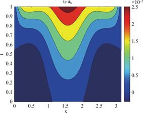
图1 h=,Δt=,α=1.7 时u-uh的等高线图
Fig.1 Contour Plot of u-uh with h=, Δt=,α=1.7
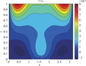
图2 h=,Δt=,α=1.7 时v-vh的等高线图
Fig.2 Contour Plot of v-vh with h=, Δt=,α=1.7
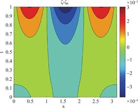
图3 h=,Δt=,α=1.7 时ζ-ζh的等高线图
Fig.3 Contour Plot of ζ-ζhwith h=,
Δt=,α=1.7
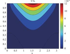
图4 h=,Δt=,α=1.2 时u-uh的等高线图
Fig.4 Contour Plot of u-uhwith h=,
Δt=,α=1.2
4.2 二维算例
在这个算例中,主要考虑一个二维的空间区域Ω=[0,1]×[0,1]及时间区域 J=[0,1],同时选择满足方程(1)初边值条件的精确解为

辅助变量为
v(x,y,t)=4t3sin(πx)sin(πy),
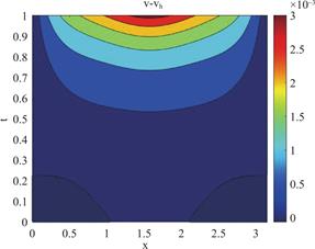
图5 h=,Δt=,α=1.2 时v-vh的等高线图
Fig.5 Contour Plot of v-vhwith h=,Δt=,α=1.2
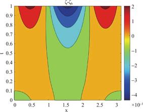
图6 h=,Δt=,α=1.2 时ζ-ζh的等高线图
Fig.6 Contour Plot of ζ-ζhwith h=,Δt=,α=1.2 ζ(x,y,t)=-2π2(1+t4)sin(πx)sin(πy),
则对应的源项为
g(x,y,t)= 12t2+4π4(t4+1)+2π2(t4+1)+
8π2t3+
 sin(πx)sin(πy)+
sin2(πx)sin2(πy).
通过固定时间步长Δt=,取定不同的时间分数阶参数α=1.1,1.3,1.5, 1.7,1.9,不同的空间步长h=1/5,1/10,1/20,1/40,在表3中记录了 u,v,ζ的L2模误差及相应的收敛结果。通过表中数据可以明显看出数值解在空间方向上的收敛阶趋近于2。
在表4中,取变化的时间分数阶参数α=1.1,1.2,1.4,1.6,1.8,变化的时空步长h=2Δt=1/20,1/30,1/40,1/50,1/60,分别给出了u,v,ζ的时间L2模误差和收敛阶。根据数据可以看出时空收敛阶依旧是趋近于2。
图7,图8和图9分别给出了h=Δt=1/100,α=1.9 时精确解与数值解之间的误差u-uh,v-vh以及ζ-ζh的等高线图。
表3 Δt= 时,u,v 和 ζ 时间误差及收敛阶
Table 3 Spatial Errors and Convergence Orders for u,v and ζ with Δt=
|
α
|
h
|
‖u-uh‖
|
Rate
|
‖v-vh‖
|
Rate
|
‖ζ-ζh‖
|
Rate
|
|
1.1
|
1/5
|
1.8423E-02
|
—
|
1.8264E-01
|
—
|
8.0957E-01
|
—
|
|
|
1/10
|
4.7115E-03
|
1.9673
|
4.4948E-02
|
2.0227
|
2.0080E-01
|
2.0114
|
|
|
1/20
|
1.1849E-03
|
1.9914
|
1.1192E-02
|
2.0058
|
5.0092E-02
|
2.0031
|
|
|
1/40
|
2.9669E-04
|
1.9978
|
2.7951E-03
|
2.0015
|
1.2517E-02
|
2.0007
|
|
1.3
|
1/5
|
1.8421E-02
|
—
|
1.7804E-01
|
—
|
8.1222E-01
|
—
|
|
|
1/10
|
4.7116E-03
|
1.9670
|
4.3796E-02
|
2.0233
|
2.0149E-01
|
2.0112
|
|
|
1/20
|
1.1850E-03
|
1.9913
|
1.0904E-02
|
2.0060
|
5.0265E-02
|
2.0030
|
|
|
1/40
|
2.9671E-04
|
1.9978
|
2.7231E-03
|
2.0015
|
1.2561E-02
|
2.0007
|
|
1.5
|
1/5
|
1.8595E-02
|
—
|
1.7113E-01
|
—
|
8.1537E-01
|
—
|
|
|
1/10
|
4.7578E-03
|
1.9665
|
4.2086E-02
|
2.0237
|
2.0230E-01
|
2.0109
|
|
|
1/20
|
1.1968E-03
|
1.9912
|
1.0477E-02
|
2.0061
|
5.0471E-02
|
2.0030
|
|
|
1/40
|
2.9966E-04
|
1.9978
|
2.6166E-03
|
2.0015
|
1.2612E-02
|
2.0007
|
|
1.7
|
1/5
|
1.9110E-02
|
—
|
1.6282E-01
|
—
|
8.1907E-01
|
—
|
|
|
1/10
|
4.8913E-03
|
1.9661
|
4.0051E-02
|
2.0233
|
2.0325E-01
|
2.0107
|
|
|
1/20
|
1.2304E-03
|
1.9910
|
9.9715E-03
|
2.0060
|
5.0709E-02
|
2.0030
|
|
|
1/40
|
3.0810E-04
|
1.9977
|
2.4903E-03
|
2.0015
|
1.2671E-02
|
2.0007
|
|
1.9
|
1/5
|
2.0196E-02
|
—
|
1.5592E-01
|
—
|
8.2327E-01
|
—
|
|
|
1/10
|
5.1696E-03
|
1.9659
|
3.8389E-02
|
2.0220
|
2.0425E-01
|
2.0110
|
|
|
1/20
|
1.3005E-03
|
1.9910
|
9.5599E-03
|
2.0056
|
5.0956E-02
|
2.0030
|
|
|
1/40
|
3.2563E-04
|
1.9977
|
2.3876E-03
|
2.0014
|
1.2733E-02
|
2.0007
|
表4 h=2Δt时,u,v和ζ的误差及收敛阶
Table 4 Errors and Convergence Orders for u,v and ζ with h=2Δt
|
α
|
h=2Δt
|
‖u-uh‖
|
Rate
|
‖v-vh‖
|
Rate
|
‖ζ-ζh‖
|
Rate
|
|
1.1
|
1/20
|
1.2224E-03
|
—
|
1.0166E-02
|
—
|
5.3846E-02
|
—
|
|
|
1/30
|
5.4178E-04
|
2.0070
|
4.7811E-03
|
1.8606
|
2.3931E-02
|
2.0001
|
|
|
1/40
|
3.0478E-04
|
1.9996
|
2.7439E-03
|
1.9301
|
1.3462E-02
|
1.9997
|
|
|
1/50
|
1.9486E-04
|
2.0047
|
1.7708E-03
|
1.9627
|
8.6166E-03
|
1.9996
|
|
|
1/60
|
1.3524E-04
|
2.0031
|
1.2343E-03
|
1.9797
|
5.9842E-03
|
1.9996
|
|
1.2
|
1/20
|
1.2213E-03
|
—
|
1.0214E-02
|
—
|
5.3708E-02
|
—
|
|
|
1/30
|
5.4089E-04
|
2.0086
|
4.7659E-03
|
1.8800
|
2.3869E-02
|
2.0001
|
|
|
1/40
|
3.0410E-04
|
2.0018
|
2.7256E-03
|
1.9424
|
1.3427E-02
|
1.9998
|
|
|
1/50
|
1.9448E-04
|
2.0033
|
1.7558E-03
|
1.9708
|
8.5940E-03
|
1.9997
|
|
|
1/60
|
1.3496E-04
|
2.0040
|
1.2226E-03
|
1.9854
|
5.9685E-03
|
1.9996
|
|
1.4
|
1/20
|
1.2237E-03
|
—
|
1.0208E-02
|
—
|
5.3424E-02
|
—
|
|
|
1/30
|
5.4215E-04
|
2.0078
|
4.6849E-03
|
1.9207
|
2.3742E-02
|
2.0002
|
|
|
1/40
|
3.0442E-04
|
2.0061
|
2.6597E-03
|
1.9680
|
1.3355E-02
|
1.9999
|
|
|
1/50
|
1.9465E-04
|
2.0042
|
1.7067E-03
|
1.9880
|
8.5477E-03
|
1.9998
|
|
|
1/60
|
1.3511E-04
|
2.0026
|
1.1857E-03
|
1.9977
|
5.9362E-03
|
1.9997
|
|
1.6
|
1/20
|
1.2383E-03
|
—
|
1.00623E-02
|
—
|
5.3129E-02
|
—
|
|
|
1/30
|
5.4927E-04
|
2.0045
|
4.53236E-03
|
1.9670
|
2.3610E-02
|
2.0003
|
|
|
1/40
|
3.0872E-04
|
2.0028
|
2.55080E-03
|
1.9982
|
1.3281E-02
|
1.9999
|
|
|
1/50
|
1.9754E-04
|
2.0010
|
1.63042E-03
|
2.0058
|
8.4999E-03
|
1.9999
|
|
|
1/60
|
1.3716E-04
|
2.0009
|
1.13624E-03
|
1.9806
|
5.9029E-03
|
1.9998
|
|
1.8
|
1/20
|
1.2857E-03
|
—
|
9.7936E-03
|
—
|
5.2816E-02
|
—
|
|
|
1/30
|
5.7012E-04
|
2.0056
|
4.3067E-03
|
2.0262
|
2.3471E-02
|
2.0003
|
|
|
1/40
|
3.2022E-04
|
2.0051
|
2.4406E-03
|
1.9742
|
1.3202E-02
|
2.0000
|
|
|
1/50
|
2.0500E-04
|
1.9988
|
1.5582E-03
|
2.0109
|
8.4495E-03
|
1.9999
|
|
|
1/60
|
1.4232E-04
|
2.0016
|
1.0837E-03
|
1.9916
|
5.8678E-03
|
1.9999
|
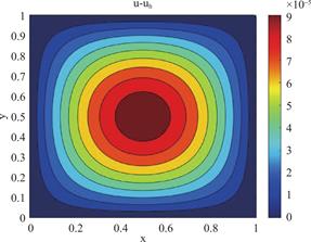
图7 h=Δt=,α=1.9 时u-uh的等高线图
Fig.7 Contour Plot of u-uhwith h=Δt=,α=1.9
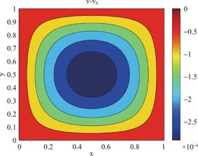
图8 h=Δt=,α=1.9 时v-vh的等高线图
Fig.8 Contour Plot of v-vhwith h=Δt=,α=1.9
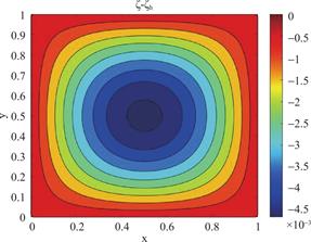
图9 h=Δt=,α=1.9 时ζ-ζh的等高线图
Fig.9 Contour Plot of ζ-ζhwith h=Δt=,α=1.9
5 结论
本文结合  格式离散时间方向,有限元方法离散空间方向,基于四阶时间分数阶双曲方程建立低阶耦合的有限元全离散格式,同时以二维区域为例给出了具体的算法过程。最后给出两个数值算例验证了数值格式的2阶收敛性。
利益冲突: 作者声明无利益冲突。
[②] *通讯作者 Corresponding author:杨益宁,yynmath@imu.edu.cn
收稿日期:2024-04-10; 录用日期:2024-04-19; 发表日期:2024-06-28
基金项目:内蒙古自治区高校创新研究团队计划(NMGIRT2413)资助。
参考文献(References)
[1] Nandal S, Pandey DN. Numerical solution of non-linear fourth order fractional sub-diffusion wave equation with time delay[J]. Applied Mathematics and Computation, 2020, 369: 124900.
https://doi.org/10.1016/j.amc.2019.124900.
[2] Ran MH, Lei XJ. A fast difference scheme for the variable coefficient time-fractional diffusion wave equations[J]. Applied Numerical Mathematics, 2021, 167: 31-44.
https://doi.org/10.1016/j.apnum.2021.04.021.
[3] Huang JF, Qiao Z, Zhang JN, Arshad S, Tang YF. Two linearized schemes for time fractional nonlinear wave equations with fourth-order derivative[J]. Journal of Applied Mathematics and Computing, 2021, 66: 561-79.
https://doi.org/10.1007/s12190-020-01449-x.
[4] Liu N, Liu Y, Li H, Wang JF. Time second-order finite difference/finite element algorithm for nonlinear timefractional diffusion problem with fourth-order derivative term[J]. Computers & Mathematics with Applications, 2018, 75: 3521-36.
https://doi.org/10.1016/j.camwa.2018.02.014.
[5] Liu Y, Du YW, Li H, He S, Gao W. Finite difference/finite element method for a nonlinear time-fractional fourthorder reaction-diffusion problem[J]. Computers & Mathematics with Applications, 2015, 70(4): 573-91.
https://doi.org/10.1016/j.camwa.2015.05.015.
[6] Liu Y, Du YW, Li H, Li JC, He S. A two-grid mixed finite element method for a nonlinear fourth-order reaction- diffusion problem with time-fractional derivative[J]. Computers & Mathematics with Applications, 2015, 70: 2474-92.
https://doi.org/10.1016/j.camwa.2015.09.012.
[7] Yang XH, Wu. LJ, Zhang. HX. A space-time spectral order sinc-collocation method for the fourth-order nonlocal heat model arising in viscoelasticity[J]. Applied Mathematics and Computation, 2023, 457: 128192.
https://doi.org/10.1016/j.amc.2023.128192.
[8] Wang JF, Yin BL, Liu Y, Li H, Fang ZC. A mixed element algorithm based on the modified L1 Crank-Nicolson scheme for a nonlinear fourth-order fractional diffusion- wave model[J]. Fractal and Fractional, 2021, 5: 274.
https://doi.org/10.3390/fractalfract5040274.
[9] Habibirad A, Hesameddini E, Shekari Y. A suitable hybrid meshless method for the numerical solution of timefractional fourth-order reaction-diffusion model in the multi-dimensional case[J]. Engineering Analysis with Boundary Elements, 2022, 145: 149-160.
https://doi.org/10.1016/j.enganabound.2022.09.007.
[10] Alikhanov AA. A new difference scheme for the time fractional diffusion equation[J]. Journal of Computational Physics, 2015, 280: 424-438.
https://doi.org/10.1016/j.jcp.2014.09.031.
[11] Wang JR, Liu Y, Wen C, Li H. Efficient numerical algorithm with the second-order time accuracy for a two-dimensional nonlinear fourth-order fractional wave equation[J]. Results in Applied Mathematics, 2022, 14: 100264.
https://doi.org/10.1016/j.rinam.2022.100264.
[12] Wang Y, Yang YN, Wang JF, Li H, Liu Y. Unconditional analysis of the linearized second-order time-stepping scheme combined with a mixed element method for a nonlinear time fractional fourth-order wave equation[J]. Computers & Mathematics with Applications, 2024, 157: 74-91.
https://doi.org/10.1016/j.camwa.2023.12.023.
[13] Fakhar-Izadi F. Fully petrov-galerkin spectral method for the distributed-order time-fractional fourth-order partial differential equation[J]. Engineering with computers[ J], 2021, 37: 2707-2716.
https://doi.org/10.1007/s00366-020-00968-2.
[14] Santra S, Behera R. A novel higher-order numerical method for parabolic integro-fractional differential equations based on wavelets and L2-1σscheme[J]. 2023, arXiv, arXiv: 2304. 08009.
https://doi.org/10.48550/arXiv.2304.08009.
L2-1σ Finite Element Method for A Nonlinear Time Fractional Fourth-order Hyperbolic Equation
WANG Yan, YANG Yining*
(School of Mathematical Sciences, Inner Mongolia University, Hohhot 010021, China)
Abstract: In this paper, a numerical algorithm with space-time second-order accuracy is constructed for a fourth-order nonlinear time fractional hyperbolic equation. Firstly, a low order parameter β =α-1 is introduced to reduce the Caputo fractional derivative ofα ∈ 1, 2 to the Caputo fractional derivative of β ∈ 0, 1 . Secondly, two auxiliary variables v=ut , ζ=Δu are introduced to transform. the fourth-order nonlinear time fractional hyperbolic equation into a low-order nonlinear coupled system with integral term. The fractional derivative term is discretized in the time direction by L2-1σ formula, and the integral term is discretized by the complex trapezoidal formula. Using the traditional Galerkin finite element method in space, the fully discrete finite element scheme of the low-order nonlinear coupling system is obtained. Taking the uniform. rectangular division on a two-dimensional region as an example, the specific forms of stiffness matrix and load matrix are given by the bilinear basis function, and the detailed algorithm implementation process of the fully discrete numerical scheme is obtained. Finally, numerical simulations are carried out for one-dimensional and two-dimensional examples. Compared with the original equation, the low-order system can observe the changes of three unknown variables u, v, ζ at the same time, and the errors, images and convergence orders of the three unknown variables are listed in detail under different parameters and different space-time steps, which fully verifies the feasibility and effectiveness of the algorithm.
Keywords: Fourth-order nonlinear time fractional hyperbolic equation, L2-1σ , Finite element method
DOI: 10.48014/fcpm.20240410001
Citation: WANG Yan, YANG Yining. L2-1σ finite element method for a nonlinear time fractional fourthorder hyperbolic equation[J]. Frontiers of Chinese Pure Mathematics, 2024, 2(2): 16-26.